


Analyzing NBA Dunks with R, a tutorial
Playing with the new NBA dunk tracking public data!

Did you know that starting from this season, the NBA is publishing data on every dunk that happens in a game? In addition to technical stats like hang time, player vertical leap, and other performance metrics, the league also assigns dunk scores ranging from 0 to at least 118—the highest recorded so far. These scores are based on four different categories, effectively turning the entire season into a dunk contest, even though the players themselves may not be aware of it.
So why wait until February and the All-Star Weekend when we can analyze dunks all year round?
The four scoring categories—Jump Score, Power Score, Style Score, and Defense Score—contribute to the final dunk rating. On top of that, the dataset includes over a dozen additional metrics, providing a unique opportunity to explore these stats in R and gain deeper insights into this newly available data from the NBA.
You can access the data directly at this link, where each dunk is accompanied by a video clip, allowing for immediate visual analysis alongside the statistics.
Let's dive into R and load the dataset to see what’s behind the numbers and how we can leverage this information for some interesting analyses!
library(tidyverse)
library(jsonlite)
library(httr)
library(janitor)

# Headers required for scraping NBA stats
headers <- c(
  `Connection` = "keep-alive",
  `Accept` = "application/json, text/plain, */*",
  `x-nba-stats-token` = "true",
  `User-Agent` = "Mozilla/5.0",
  `x-nba-stats-origin` = "stats",
  `Referer` = "https://stats.nba.com/players/leaguedashplayerbiostats/",
  `Accept-Encoding` = "gzip, deflate, br",
  `Accept-Language` = "en-US,en;q=0.9"
)

# Prevent connection error
Sys.setenv("VROOM_CONNECTION_SIZE" = 131072 * 2)

# NBA Dunks Leaderboard Data URL
url <- "https://stats.nba.com/stats/dunkscoreleaders?LeagueID=00&Season=2024-25&SeasonType=Regular%20Season"

# Fetch and process data
res <- GET(url, add_headers(.headers = headers))
json_resp <- fromJSON(content(res, "text"))
dunks <- as_tibble(json_resp$dunks) %>%
  clean_names()
As you'll soon notice, there are numerous hidden columns that only become available once you download the table locally. These include details about the passer, dunk type (e.g., 360, windmill, etc.), jumping foot, dunking hand, and even the pass location—all valuable information for our analysis.
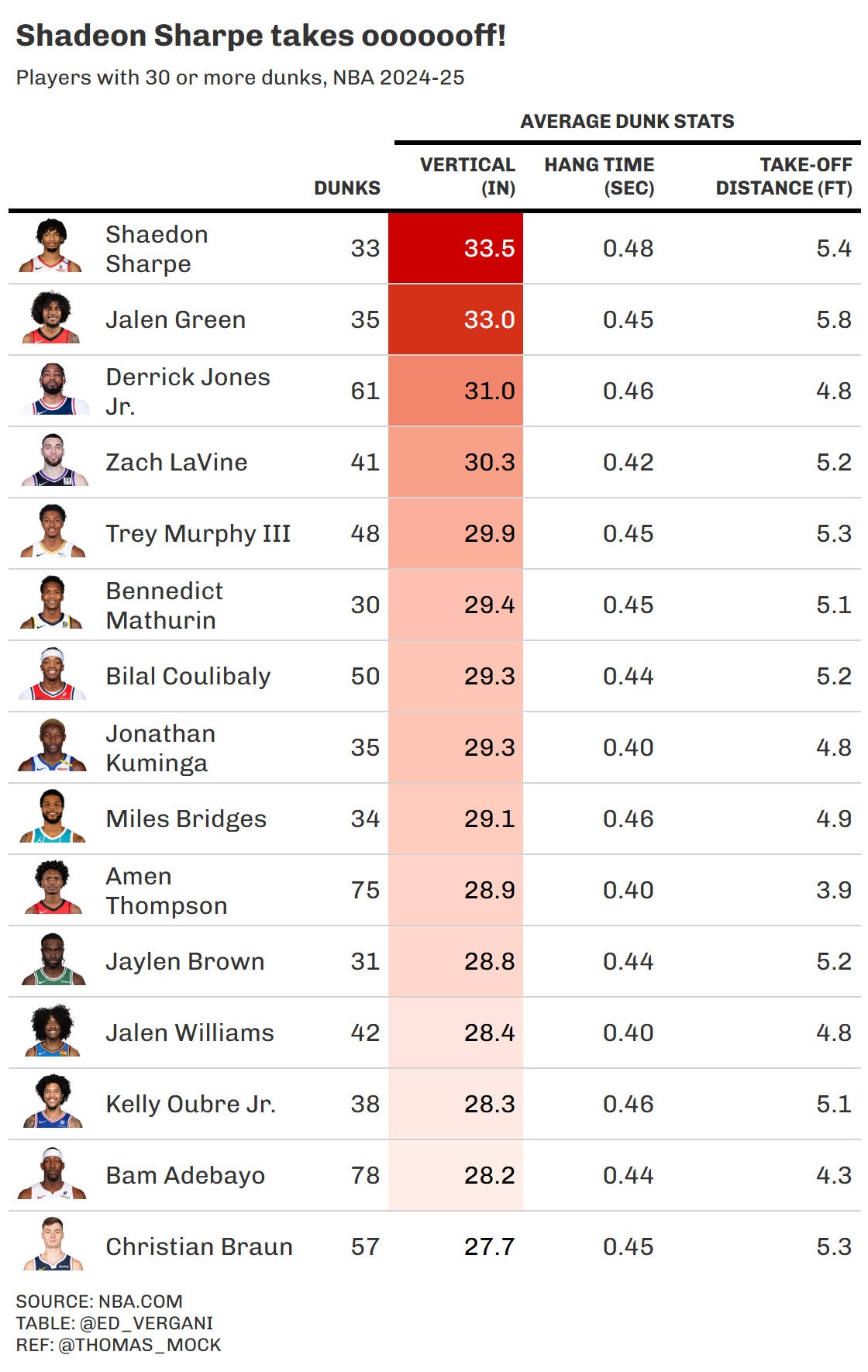
Let’s start with something simple: calculating average dunk scores for players who have performed at least 30 dunks throughout the season.
averages <- dunks %>%
  group_by(player_id, player_name) %>%
  summarise(
    dunks = n(),
    avg_player_vertical = mean(player_vertical, na.rm = TRUE),
    avg_hang = mean(hang_time, , na.rm = TRUE),
    avg_distance = mean(takeoff_distance, na.rm = T)
  )%>%
  filter(dunks>=30)
The expected output from this table will be a summary of average dunk scores for players with at least 30 dunks during the season.

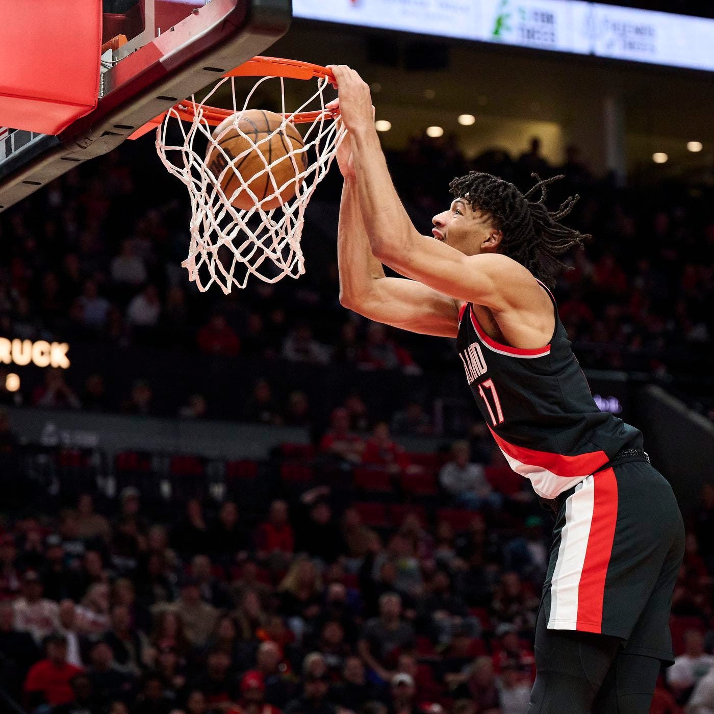
Finally, we have objective proof of what an incredible athlete Shaedon Sharpe is!
On average, he reaches 33.5 inches (about 88 cm) in vertical leap, maintains half a second of hang time, and takes off from 5.35 feet (1.60 meters) away from the basket.
Now, let’s clean things up and make our table more presentable, leveraging the excellent gt package in R. We'll also take advantage of some custom styling code by Thomas Mock, which allows us to format our table with a FiveThirtyEight-style aesthetic.
For the table theme, I’ve directly adapted the code from Thomas’ blog post. Let’s apply it and refine our output!
gt_theme_538 <- function(data,...) {
  data %>%
    opt_all_caps()  %>%
    opt_table_font(
      font = list(
        google_font("Chivo"),
        default_fonts()
      )
    ) %>%
    tab_style(
      style = cell_borders(
        sides = "bottom", color = "transparent", weight = px(2)
      ),
      locations = cells_body(
        columns = TRUE,
        # This is a relatively sneaky way of changing the bottom border
        # Regardless of data size
        rows = nrow(data$`_data`)
      )
    )  %>%
    tab_options(
      column_labels.background.color = "white",
      table.border.top.width = px(3),
      table.border.top.color = "transparent",
      table.border.bottom.color = "transparent",
      table.border.bottom.width = px(3),
      column_labels.border.top.width = px(3),
      column_labels.border.top.color = "transparent",
      column_labels.border.bottom.width = px(3),
      column_labels.border.bottom.color = "black",
      data_row.padding = px(3),
      source_notes.font.size = 12,
      table.font.size = 16,
      heading.align = "left"
    )
}
I can't stress enough how great Thomas and his website are for anyone working with gt tables, or when you need to incorporate images into plots and tables! If you haven't already, go check out his work—it's a goldmine of useful techniques for data visualization in R!
image_df = nba_players()
image_df = image_df %>%
  select(idPlayer, urlPlayerHeadshot)

vertical = merge(vertical, image_df, by.x = "player_id", by.y = "idPlayer")

dunks <- vertical %>%
  arrange((-avg_player_vertical)) %>%
  head(15) %>%
  mutate(avg_player_vertical = round(avg_player_vertical, 1),
         avg_hang  = round(avg_hang , 2),
         avg_distance = round(avg_distance, 1)) %>%
  select(urlPlayerHeadshot, player_name, dunks, avg_player_vertical, avg_hang, avg_distance) %>%
  gt()  %>%
  tab_spanner(
    label = "AVERAGE DUNK STATS",
    columns = 4:6
  ) %>%
  tab_header(
    title = md("**Shadeon Sharpe takes ooooooff!**"),
    subtitle = md("Players with 30 or more dunks, NBA 2024-25")
  ) %>%
  data_color(
    columns = vars(avg_player_vertical),
    colors = scales::col_numeric(
      palette = c("white", "#cc0000"),
      domain = NULL
    )
  ) %>%
  cols_label(
    urlPlayerHeadshot = '',
    player_name = '',
    dunks = 'DUNKS',
    avg_player_vertical = 'VERTICAL (IN)',
    avg_hang = 'HANG TIME (SEC)',
    avg_distance = 'TAKE-OFF DISTANCE (FT)'
  ) %>%
  tab_source_note(
    source_note = md("SOURCE: NBA.COM <br> TABLE: @ED_VERGANI <br> REF: @THOMAS_MOCK")
  ) %>%
  text_transform(
    locations = cells_body(urlPlayerHeadshot),
    fn = function(x) {
      web_image(url = x, height = 35)
    }
  ) %>%
  gt_theme_538(table.width = px(550))


gtsave(dunks, filename = "Dunks.png")
The incredible result will be a polished and visually appealing table displaying the top NBA dunkers who have performed at least 30 dunks during the season:
Let's continue our dunk analysis with another interesting insight: the average pass length for alley-oops among players who have assisted the most dunks.
Since this analysis is similar to the previous one, the code structure remains largely the same. Here’s how we can do it in R:
passer <- dunks %>%
  group_by(passer_name, passer_id) %>%
  summarise(
    dunks_assisted = n(),
    avg_pass_length = mean(pass_length, na.rm = TRUE)
  )%>%
  filter(dunks_assisted>=10 & passer_id != 0)

passer = merge(passer, image_df, by.x = "passer_id", by.y = "idPlayer")

pass_table <- passer %>%
  arrange((-avg_pass_length)) %>%
  head(15) %>%
  mutate(dunks_assisted = round(dunks_assisted, 1),
         avg_pass_length  = round(avg_pass_length , 1)) %>%
  select(urlPlayerHeadshot, passer_name,  dunks_assisted, avg_pass_length) %>%
  gt()  %>%
  tab_header(
    title = md("**Alley-oop pass masters**"),
    subtitle = md("Players with 10 or more dunks assisted, NBA 2024-25")
  ) %>%
  data_color(
    columns = vars(avg_pass_length),
    colors = scales::col_numeric(
      palette = c("white", "#cc0000"),
      domain = NULL
    )
  ) %>%
  cols_label(
    urlPlayerHeadshot = '',
    passer_name = '',
    dunks_assisted = 'DUNKS ASSISTED',
    avg_pass_length = 'AVG PASS LENGTH (FT)',
  ) %>%
  tab_source_note(
    source_note = md("SOURCE: NBA.COM <br> TABLE: @ED_VERGANI <br> REF: @THOMAS_MOCK")
  ) %>%
  text_transform(
    locations = cells_body(urlPlayerHeadshot),
    fn = function(x) {
      web_image(url = x, height = 35)
    }
  ) %>%
  gt_theme_538(table.width = px(400))

gtsave(pass_table, filename = "DunksPassers.png")
Look at LaMelo, man, so inspirational!

Finally, let's take a look at the most dominant alley-oop duos in the NBA!
We'll analyze which passer-dunker pairs have connected for the most alley-oops, ranking them by total dunks assisted, average pass distance and average vertical leap for those plays.
most_frequent <- dunks %>%
  group_by(passer_name, passer_id, player_name, player_id) %>%
  summarise(
    dunks_assisted = n(),
    avg_pass_length = mean(pass_length, na.rm = TRUE),
    avg_player_vertical = mean(player_vertical, na.rm = TRUE)
  )%>%
  filter(dunks_assisted>=10 & passer_id != 0)

most_frequent = merge(most_frequent, image_df, by.x = "passer_id", by.y = "idPlayer")
most_frequent = merge(most_frequent, image_df, by.x = "player_id", by.y = "idPlayer")

duo_table <- most_frequent %>%
  arrange((-dunks_assisted)) %>%
  head(15) %>%
  mutate(dunks_assisted = round(dunks_assisted, 1),
         avg_pass_length  = round(avg_pass_length , 1),
         avg_player_vertical = round(avg_player_vertical, 1)) %>%
  select(urlPlayerHeadshot.x, passer_name,, urlPlayerHeadshot.y, player_name, dunks_assisted, avg_pass_length, avg_player_vertical) %>%
  gt()  %>%
  tab_spanner(
    label = "AVERAGE DUNK STATS",
    columns = 6:7
  ) %>%
  tab_header(
    title = md("**Alley-oop duos!**"),
    subtitle = md("Duos with 10 or more dunks in passer-dunker combo, NBA 2024-25")
  ) %>%
  data_color(
    columns = vars(dunks_assisted),
    colors = scales::col_numeric(
      palette = c("white", "#cc0000"),
      domain = NULL
    )
  ) %>%
  data_color(
    columns = vars(avg_pass_length),
    colors = scales::col_numeric(
      palette = c("white", "blue"),
      domain = NULL
    )
  ) %>%
  data_color(
    columns = vars(avg_player_vertical),
    colors = scales::col_numeric(
      palette = c("white", "orange"),
      domain = NULL
    )
  ) %>%
  cols_label(
    urlPlayerHeadshot.x = '',
    passer_name = 'FROM...',
    urlPlayerHeadshot.y = '',
    player_name = '...TO',
    dunks_assisted = 'DUNKS ASSISTED',
    avg_pass_length = 'PASS LENGTH (FT)',
    avg_player_vertical = 'VERTICAL (IN)'
  ) %>%
  tab_source_note(
    source_note = md("SOURCE: NBA.COM <br> TABLE: @ED_VERGANI <br> REF: @THOMAS_MOCK")
  ) %>%
  text_transform(
    locations = cells_body(urlPlayerHeadshot.x),
    fn = function(x) {
      web_image(url = x, height = 35)
    }
  ) %>%
  text_transform(
    locations = cells_body(urlPlayerHeadshot.y),
    fn = function(x) {
      web_image(url = x, height = 35)
    }
  )   %>%
  gt_theme_538(table.width = px(650))

gtsave(duo_table, filename = "DunksDuos.png")
The Cade - Jalen duo is really above everyone else in the NBA!

Ora, torniamo a parlare dei punteggi citati prima, e creiamo un’altra tabella riassuntiva.
scores <- dunks %>%
  group_by(player_name, player_id) %>%
  summarise(
    dunks = n(),
    dunk_score = mean(dunk_score, na.rm = TRUE),
    jump_subscore = mean(jump_subscore, , na.rm = TRUE),
    power_subscore = mean(power_subscore, na.rm = TRUE),
    style_subscore = mean(style_subscore, na.rm = T),
    defensive_contest_subscore = mean(defensive_contest_subscore , na.rm = TRUE),
  )%>%
  filter(dunks>=30)

scores = merge(scores, image_df, by.x = "player_id", by.y = "idPlayer")


scores_table <- scores %>%
  arrange((-dunk_score)) %>%
  head(15) %>%
  mutate(dunk_score = round(dunk_score, 1),
         jump_subscore  = round(jump_subscore , 1),
         power_subscore = round(power_subscore, 1),
         style_subscore = round(style_subscore, 1),
         defensive_contest_subscore = round(defensive_contest_subscore, 1)
         ) %>%
  select(urlPlayerHeadshot, player_name, dunks, dunk_score, jump_subscore, power_subscore, style_subscore, defensive_contest_subscore) %>%
  gt()  %>%
  tab_spanner(
    label = "AVERAGE DUNK SCORES",
    columns = 4:8
  ) %>%
  tab_header(
    title = md("**Dunk Wars: The Ultimate Year-Round Dunk Contest!**"),
    subtitle = md("Players with 30 or more dunks, scores via NBA website")
  ) %>%
  tab_style(
    style = list(
      cell_text(weight = "bold")
    ),
    locations = cells_body(
      columns = 4
    )
  ) %>%
  tab_style(
    style = list(
      cell_text(weight = "bold")
    ),
    locations = cells_body(
      columns = jump_subscore,
      rows = jump_subscore > mean(jump_subscore)*1.2
    )
  )%>%
  tab_style(
    style = list(
      cell_text(weight = "bold")
    ),
    locations = cells_body(
      columns = power_subscore,
      rows = power_subscore > mean(power_subscore)*1.2
    )
  )%>%
  tab_style(
    style = list(
      cell_text(weight = "bold")
    ),
    locations = cells_body(
      columns = style_subscore,
      rows = style_subscore > mean(style_subscore)*1.2
    )
  )%>%
  tab_style(
    style = list(
      cell_text(weight = "bold")
    ),
    locations = cells_body(
      columns = defensive_contest_subscore,
      rows = defensive_contest_subscore > mean(defensive_contest_subscore)*1.2
    )
  )%>%
  data_color(
    columns = vars(dunk_score),
    colors = scales::col_numeric(
      palette = c("white", "#d7191c"),
      domain = NULL
    )
  )%>%
  cols_label(
    urlPlayerHeadshot = '',
    player_name = '',
    dunks = 'DUNKS',
    dunk_score = 'DUNK SCORE', jump_subscore = 'JUMP', power_subscore = 'POWER', style_subscore = 'STYLE', defensive_contest_subscore = ' DEF. CONTEST'
  ) %>%
  tab_source_note(
    source_note = md("SOURCE: NBA.COM <br> TABLE: @ED_VERGANI <br> REF: @THOMAS_MOCK")
  ) %>%
  text_transform(
    locations = cells_body(urlPlayerHeadshot),
    fn = function(x) {
      web_image(url = x, height = 35)
    }
  ) %>%
  gt_theme_538(table.width = px(550))

gtsave(scores_table, filename = "DunksScores.png")
Look how amazing our year long dunk contest looks:

Jalen Green’s dunks are looking amazing!